


“So, which of our customers are likely to buy again?”
It’s a common question you may hear during your weekly marketing meeting. But too often, the answer gets buried with technical jargon like logistic regression, gradient boosting, or ML pipelines. While these are all valid techniques, you don’t always need complex models to build a useful, production ready propensity model.
Propensity modeling predicts the likelihood of a customer taking some action. In this case, it is coming back to make another purchase. By understanding who is likely to come back and purchase, marketing teams are able to retarget wisely, prioritize offers, and send the right message at the right time.
In this blog, I walk you through how you can build a simple, quick, and effective propensity model. All you need is a data warehouse, any notebook, and python/SQL. If you’re an analytics engineer running propensity analysis for the first time, the following framework will help get you started:
First and foremost, you want to start with a hypothesis for why someone is likely to buy again. Does it have to do with when a customer purchases (seasonality, holidays, etc.), how much a customer spends, how many items are purchased, or how much time passes between orders? Choosing the right features is a balance of what data is available and grouping features with similarities.
By having a hypothesis in place, you are able to have a narrow focus on what to test. With an alignment of data inputs with your hypothesis, you are likely to have stronger signals for repurchase and better model outcomes. This is opposed to looking at everything, seeing what sticks, and getting lost in what can be meaningful features for repurchase. Where possible, it is also recommended to collaborate with your stakeholders on different hypothesis they are interested in testing.
Once the hypotheses have been established, it is time to build and explore your dataset. Our dataset relies heavily on Shopify and what is available across order, customer and product tables. This includes customer details (ID, First Purchase Date, Repeat Purchase Date, State/Province, Country, etc.), transactional details about a customer’s first order (order value, number of items purchased, unique products purchased, days between orders, etc.) and our target variable (did the customer order again).
With the dataset established, it is time to explore the timeframe for which someone is likely to repurchase and separate timing from propensity, i.e. distinguish if a customer will repurchase from when they will repurchase. To do so, we use a cumulative distribution to find when 95% of repeat purchases occur. Note that outliers will not dramatically impact the distributed view if the number of days to repurchase is very large. This is because the cumulative distribution function (CDF) tends to impact the tail end, while the central portion of the data remains unchanged.
By determining when 95% of repeat purchases occur, we are able to define buckets for propensity (very likely, likely, moderate, unlikely, very unlikely). These buckets help prioritize engagement with customers based on where they fall in the repurchase timeline. Additionally, this helps to determine how much data is “cut out” when we begin testing our features.
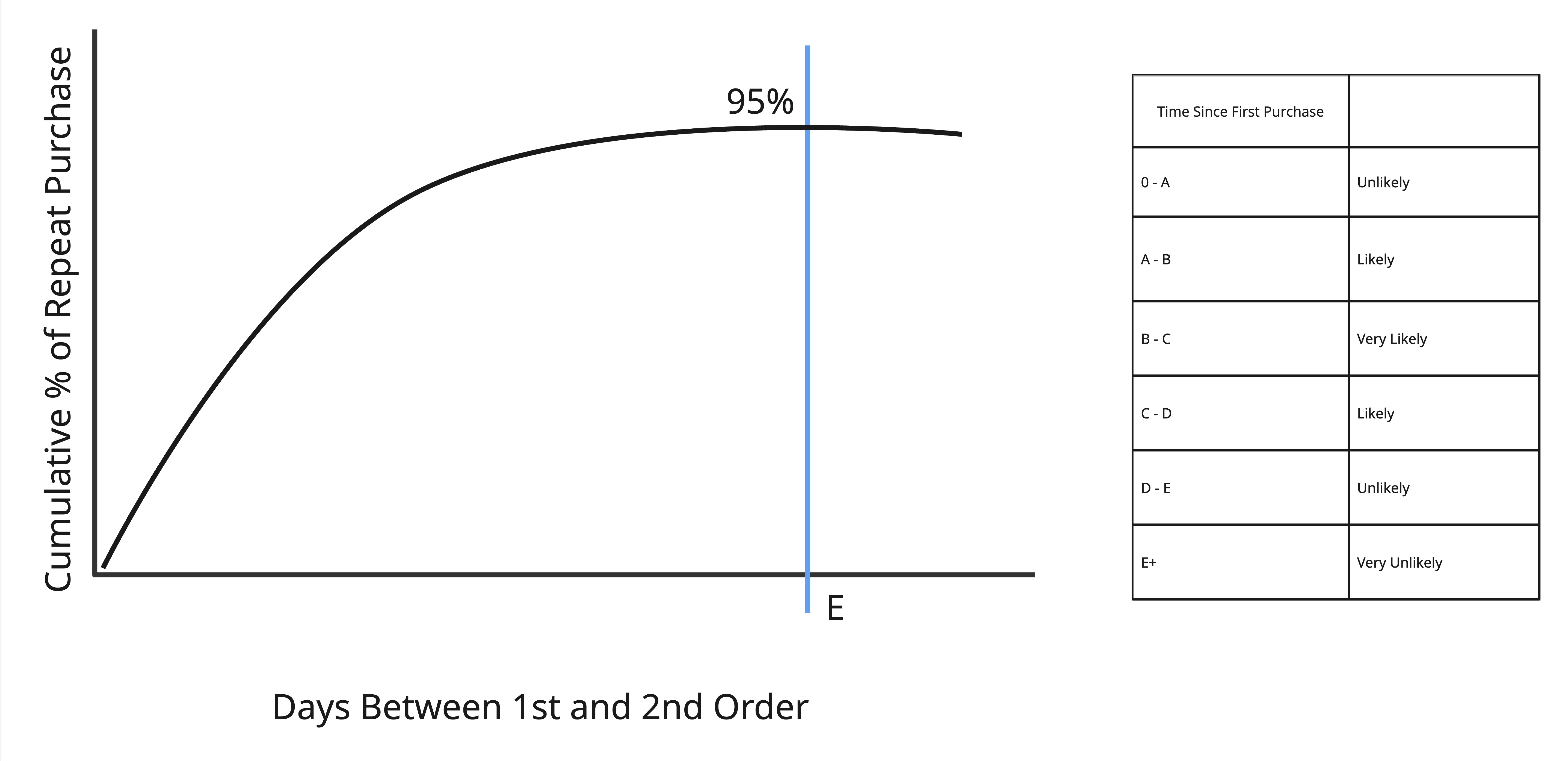
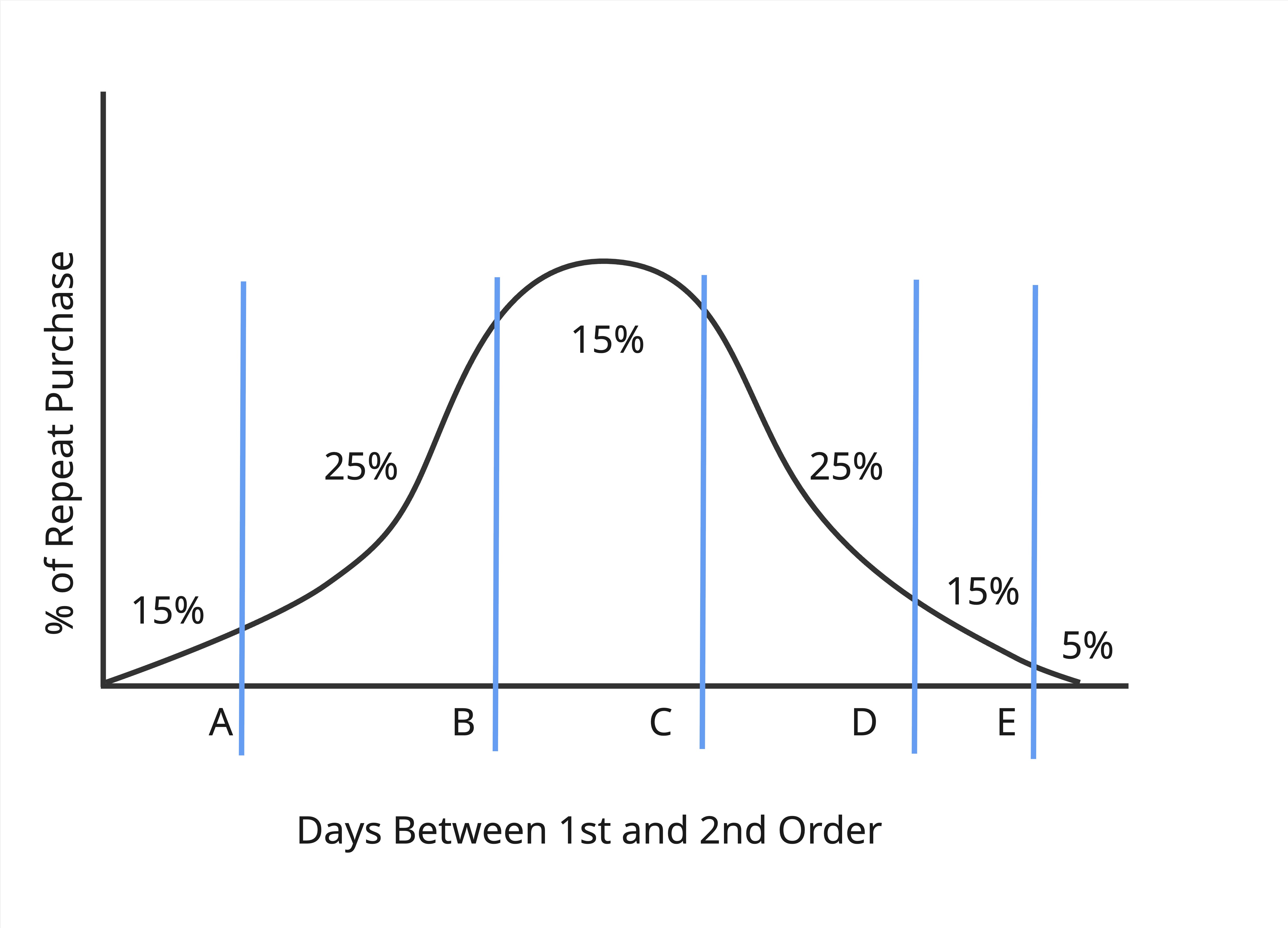
Our findings show that 95% of customers repeat within 843 days. Based on these results, we need to remove approximately two years of data from our testing set. We should explore this further to identify key patterns to potentially reduce the cutoff % to be lower (75% or 80%). To do so, we plot a distribution for when people are repurchasing and find it is skewed to the right. So for the tail, further investigation is done to see if customers are waiting for discount or holiday sales such as Black Friday.
The data shows that there are in fact cyclical spikes during the holiday (November) season. This suggests that people are waiting for the holidays to make a purchase/repurchase. These customers are removed from the cumulative distribution chart. When re-plotting the CDF, we find that the cut off date has not changed much at 800 days. So, the cutoff criteria is lowered to 75%.
For 75% of customers, repurchase is done within 308 days of their first order. Additional buckets are created as follows:
Now we can test our features and use the 308-day window as the cut off period for testing and training our data.
At a high level, the approach used is as follows:
There are many approaches for testing statistical significance (Univariate Logistic Regression, Point-Biserial Correlation, Area Under the Curve, etc.). However, as mentioned earlier, the goal here is to start simple. Given the nature of the features being tested, we can use a chi-square test. Chi-square tests are very effective in testing binary outcomes (compared to say if you were analyzing how much a customer is likely to spend given that it is a holiday period).
To run the chi-square test, we bucket non-categorical data into logical groups. Note that logical here can be determined by plotting the distribution first, then assigning groups based on that. Plot the bucketed-data vs the outcome variable (% repeat). Note any differences in the % repeat rate for each bucket, and re-bucket as needed to exaggerate the differences in groups. Then, run a chi-square test to determine statistical significance. Essentially, the chi-square test is telling us the likelihood of the observed differences in each group being due to chance. The chi-square test will return a p-value. If the p-value is less than 0.05, this means the feature is statistically significant and a likely indicator for a customer making a repeat purchase.
After testing each feature, run a correlation test between them. This will help determine which features are the same and narrow down your list of features. This helps to ensure that the interpretation of results and reasons for repurchasing are clear, reduce noise, and improve model accuracy.
In this instance, features like whether it is a holiday or if a user purchased multiple items are a predictor for if someone will purchase again.
Pairing the cut-off period with our features, it is time to productize our findings. We start with a weighted scoring in SQL. A weight is applied to each bucket of days since first purchase. A smaller weight is applied to multi-item purchases and a holiday purchases. A sum of the weights is used to produce a total score for each customer. This score is then used to determine the propensity flag (very likely, likely, moderate, unlikely, very unlikely) for each customer.
To set up your training set for the propensity classification, start by identifying all first-time purchases prior to your cutoff date (in this case, 308 days ago). This will create a snapshot of users who made their first purchase and those who had not yet purchased as of the cutoff. Next, determine which users completed a second purchase. Exclude any users whose second purchase occurred before the snapshot date. This process leaves you with a training set of customers who had not yet made a second purchase, along with a flag indicating whether they returned after the snapshot date. This flag will help validate that the propensity classification is working as intended.
Weighted scoring is an iterative process. The goal is to assess how many customers fall into each propensity group, but also ensure that each group has a very different repeat % from one another. Meaning, we should see that the unlikely group has a lower % repeat when comparing to moderate and likely groups. Ideally, very likely has the highest % repeat and very unlikely the lowest % repeat.
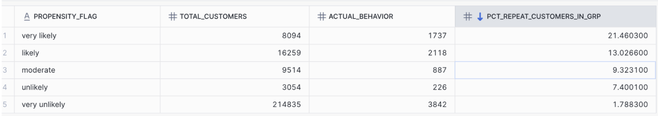
To view these observations, examine the total number of customers in each group, as defined by the total score outlined above. Compare this to the actual behavior observed, determined by the flag indicating whether a customer repurchased after the snapshot date. The screenshot below illustrates the customer count per group, their actual behavior, and the percentage deviation for each propensity flag. As expected, the groups show distinct percentages, suggesting that our scoring is working well.
By taking a simple approach to propensity modeling, our team was able to work quickly and provide a focused approach for whether a customer is likely to repurchase.
Note that this analysis is certainly not complete but rather ongoing. Why? Things change in customer behavior all the time and for any reason. This means having to periodically re-evaluate your features to see what is still relevant and significant for a customer’s propensity.
Additionally, as business needs arise, you may consider building in more sophistication for the model, such as logistical regressions or autonomous updates for features based on new behaviors in the data.
The most important thing is to start with a hypothesis, start simple, and think about what the business needs in its current state with its current data. By breaking down propensity modeling in this way, you’ll be able to help your team take action by targeting the right customers at the right time.